User Manual for Materials Consumption Simulator
中文版
物料消耗模拟器用户指南Materials Consumption Simulator
Materials Consumption Simulator1. Why Simulate
1.1. The Base Scenario C0
Imagine you are the Project Manager (PM) overseeing a single-center randomized controlled trial (RCT). The trial design is presented in Figure 1.
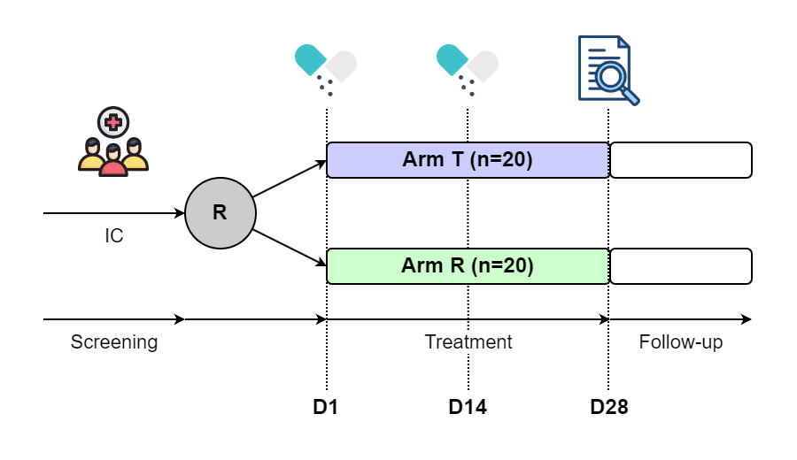
Figure 1. Base Scenario C0
The trial protocol specifies that 40 patients who meet the inclusion and exclusion criteria will be randomized into two treatment arms: Arm T and Arm R, with an allocation ratio of 1:1. Each patient will receive two kits of materials, one on Day 1 and one on Day 14.
The theoretical consumptions of materials is relatively straightforward to calculate:
For T:
20 patients × 2 kits/patient (at Day 1 and 14) = 40 kits
For R:
20 patients × 2 kits/patient (at Day 1 and 14) = 40 kits
Since this is a single-center trial, it is relatively straightforward for you, as the PM, to ensure that the correct amount of materials are shipped to the center. In this case, you can justify that at least 40 kits of T and 40 kits of R should be shipped to the center to cover the expected consumption. However, to account for potential unforeseen circumstances, you decide to add a small buffer. Based on your experience and historical data, you anticipate a 5% chance of re-dispense due to various factors such as:
- Kit damage
- Loss during shipment
- Patient non-compliance or errors in dosing
To mitigate the risk of running out of materials, you decide to ship an additional 5% of the original required amount for each arm. This results in 42 kits for T and 42 kits for R.
C0 is a clear example of how, in trials with simple logistics and predictable needs, a manual approach can be sufficient, making simulations unnecessary for material supply planning.
1.2. The Alternative Scenarios Ccenter=2
You’re facing significant pressure to advance the timeline of your trial. To accelerate patient accrual, you decide to expand from a single-center to a multi-center RCT. Now, you have two centers to manage. The key question becomes:
-
How can you predict material consumption for a trial with multiple centers like Ccenter=2?
Let’s break down the questions and challenges you're likely facing:
Central Randomization and Patient Enrollment Distribution
Under the framework of central randomization, patients are randomly assigned to either Arm T or Arm R. Since the total number of patients across all centers is fixed at 40, there are 41 possible enrollment outcomes for the two centers—ranging from 0 to 40 patients being enrolled at Center 1, with the remaining patients assigned to Center 2. Each outcome results in a different combination of patients in each arm at both centers.
Uncertainty in Material Requirements
Given the uncertainty in how patients will be distributed across the centers, it’s challenging to accurately predict how many materials should be shipped to each center.
The simplest, most conservative approach might be to send 40 kits of T and 40 kits of R to both centers. However, this will lead to overstocking at all centers. The actual material consumption could end up being 200% of the theoretical amount, which would significantly increase costs and resource wastage — an unacceptable outcome.
To avoid overstocking and reduce unnecessary waste, you consider an alternative strategy: Ship 30 kits of T and 30 kits of R to each center. This ensures that materials are distributed more reasonably, and the consumption would increase to only 150% of the theoretical consumption (rather than 200%). While this approach is still more than the minimum needed, it offers a more balanced solution, covering potential variations in patient enrollment without excessive overstock.
In Real World
Instead of shipping all the materials at once, you consider a more adaptive shipping strategy. This allows you to adjust material shipments based on the actual enrollment status of each center over time, reducing the risk of either overstocking or running out of materials. Here’s how it could work:
- Initial Supply: Based on the expected patient enrollment, you ship a smaller quantity of materials to each center, for example, 10 kits of T and 10 kits of R to each center. This takes into account the early patient enrollment and ensures you without overstocking.
- Re-supply: As patient enrollment progresses, you monitor the actual consumption at each center. When inventory levels drop below a certain threshold, a re-supply is triggered. The threshold is the minimum stock level that ensures you don’t run out of materials between shipments.
Of course, you have to specify follow parameters:
- How many kits should be shipped to each center for the first shipment?
- What is the threshold for stock to trigger subsequent shipments?
- How many kits should be shipped for subsequent shipments?
1.3. Quick View of Simulation
This is where simulation becomes invaluable. By using simulation, you no longer need to rely on simple, deterministic calculations. The simulation accounts for the uncertainty in how patients will be distributed across the centers and how materials will be consumed. With this approach, you can identify the optimal supply strategy that balances the need to ensure adequate supply without excessive overstocking or stockouts. And you can make data-driven decisions that improve the accuracy and efficiency of your clinical trial logistics.
At this stage, we understand that diving into the details of how to carry out a simulation might seem overwhelming, so we will focus on presenting the key evaluation results directly:
Table 1. Various Supply Strategy
| # | Supply Strategy | Coverage | Theoretic Consumption |
Actual Consumption |
Inflation Ratio |
|---|---|---|---|---|---|
| 1 | Single Shipment of 40 Ts and 40 Rs | 100% | 40 Ts and 40 Rs | 80 Ts and 80 Rs | 200.0% |
| 2 | Single Shipment of 30 Ts and 30 Rs | 99% | 40 Ts and 40 Rs | 60 Ts and 60 Rs | 150.0% |
| 3 | Multiple Shipment with Initial 20 Ts and 20 Rs Supply 5 Ts and 5 Rs if any stock is under 5 |
99% | 40 Ts and 40 Rs | 57 Ts and 57 Rs | 142.5% |
| 4 | Multiple Shipment with Initial 10 Ts and 10 Rs Supply 5 Ts and 5 Rs if any stock is under 5 |
98% | 40 Ts and 40 Rs | 56 Ts and 55 Rs | 137.5% |
| 5 | Multiple Shipment with Initial 10 Ts and 10 Rs Supply adaptively if any stock is under 5 |
96% | 40 Ts and 40 Rs | 50 Ts and 50 Rs | 122.5% |
The short answer is that Scenario #4 or Scenario #5 are the most recommended options, with actual material consumption predicted to be between 123% and 138% of the theoretical consumption. This range provides a more realistic estimate of the materials required, and is much more efficient than preparing 150% or even 200% of the materials, which would lead to overstocking and unnecessary costs.
In the following sections, MACROLIB will walk you through the underlying mechanisms of the Monte Carlo simulation used to model materials consumption. We’ll cover:
- How the simulation works: A detailed explanation of the Monte Carlo method and how it is applied to predict material usage across various trial scenarios.
- Setting up the simulation: A practical guide on how to define and justify the simulation parameters to ensure accurate predictions for your specific trial needs.
- Interpreting the results: A step-by-step explanation of how to interpret the outputs from the simulation, including insights on what the results mean for your materials supply strategy.
Finally, we will introduce the Warehouse: a collection of advanced examples that demonstrate real-world use cases and simulation outcomes. These examples will serve as a reference, helping you better understand how to apply the simulation in different trial contexts.
2. How to Simulate
Here’s a quick and easy version to help you explain the idea to your colleagues without getting bogged down in technical details:
- MACROLIB utilizes Monte Carlo Simulation to understand the impact of uncertainty in predictions by running multiple iteration with different scenarios. Each iteration is a trial run that adjusts the variables randomly, simulating different possible outcomes.
By repeating these simulations many times (often thousands of iterations), instead of relying on a single, potentially inaccurate estimate, you get a range of possible outcomes, which helps you make more informed decisions — you’re not just guessing; evidence is based on a wide range of potential scenarios.
If you’re the type who likes to get into the technical details and really understand how it all works under the hood, don’t worry — we’ve got you covered. The following sections will break down the Monte Carlo simulation process in plain English, so even if you don’t have a background in statistics, you can still follow along and get a solid grasp of how the simulations work and how to interpret the results.
2.1. Objective Function
A robust material supply strategy should primarily address:
Determining the Optimal Supply Strategy - Balance between Outstock and Overstock.
One side is ensuring that each center has enough stock available to meet the needs of patients when they visit to claim their study materials. This is essential to maintaining trial integrity, as failure to dispense materials according to the protocol can have serious consequences.
However, the other side is avoiding overstocking at centers. While ensuring that sufficient stock is available is crucial, overstocking can be equally problematic. Excessive stock levels at centers lead to wastage and inefficiency.
Additionally, depending on the context, other factors should be carefully eluvated:
- For products with strict storage conditions (e.g., those requiring temperature control or humidity regulation), the optimal strategy might be one that minimizes the number of shipments to reduce the complexity of storage management.
- For products with a short shelf life, the optimal strategy might focus on minimizing stock levels at any given time. The aim would be to avoid having large amounts of material sitting in inventory for too long, reducing the risk of expired stock.
In each case, optimality is about balancing the trade-offs between availability, cost, storage complexity, and product life cycle. Depending on the specific product and trial requirements, the optimal strategy may prioritize one or more of these factors.
2.2. Complex System
In the real world, clinical supply chains don’t operate in isolation. They are shaped by multiple dimensions that constantly interact with each other.
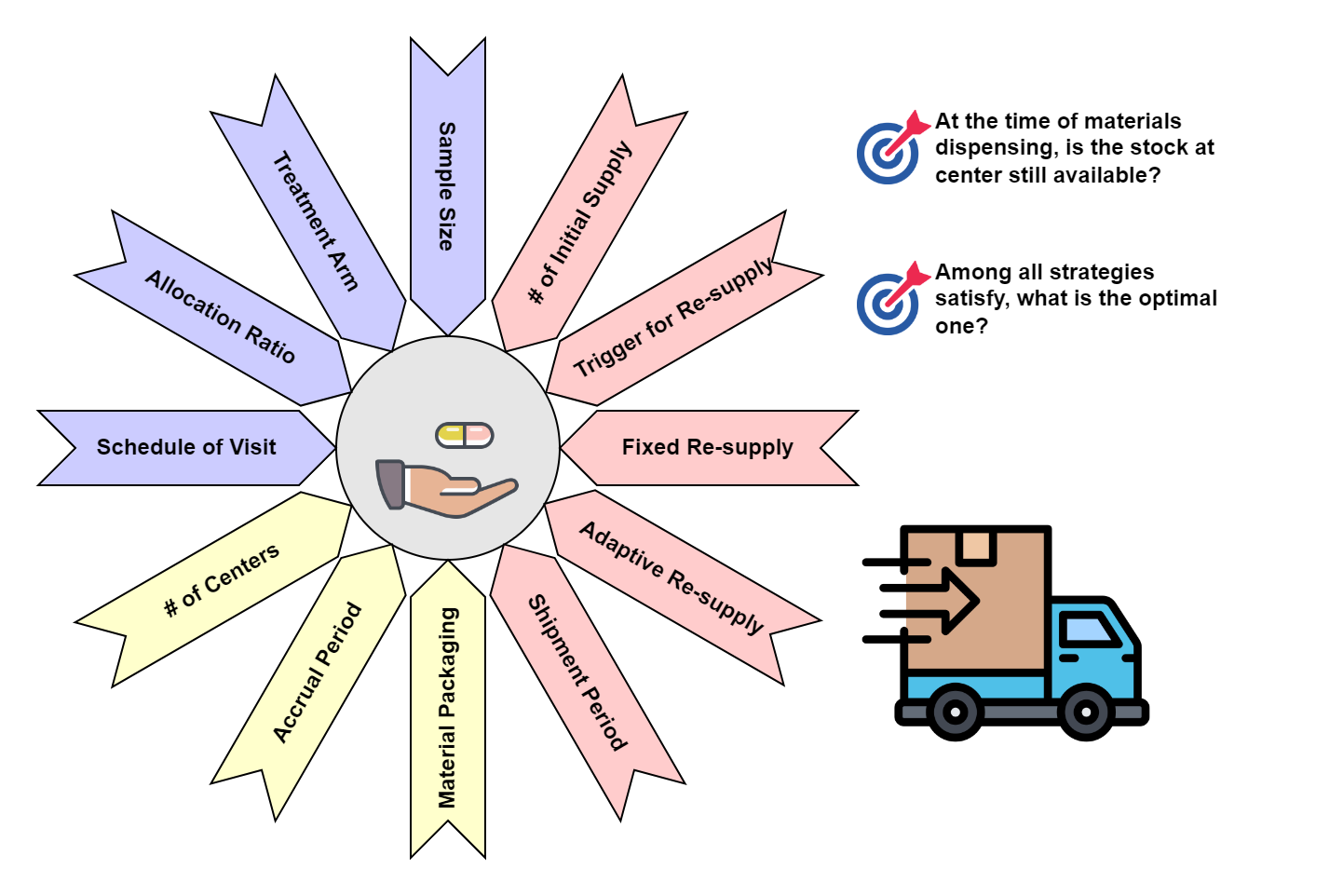
Figure 3. Complex System for Clinical Trial Material Supply
These dimensions include:
- Trial design is the foundational dimension that directly affects supply planning. As we discussed in Section 1.1, the theoretical consumption of materials is derived from factors such as sample size, treatment arm allocation, and visit schedule. These factors are crucial in calculating the base amount of materials needed for the trial.
- The logistics of your trial also play a critical role in determining the supply strategy. In Section 1.2, we illustrated how adding another center can impact material distribution. But logistics isn’t just about the number of sites. Other factors, like patient accrual rates, shipping time, and inventory turnover, also introduce complexities.
Once both the trial design and logistics are finalized, the supply strategy can be formulated to ensure the right amount of materials are available at the right time. we can apply different strategies to manage material distribution and resupply. For example, Table 1 (provided later in this section) illustrates various supply strategies for a multi-center trial (Ccenter=2).
Take Supply Strategy #4 as an exmple:
When the stock reaches the re-supply threshold of 5 kits, a shipment is initiated.
Each re-supply shipment includes 5 kits of T and 5 kits of R for the center in need.
This re-supply arrives within 3 days, ensuring that the center has the materials they need to continue dispensing without interruptions.
In this scenario, multiple shipments are planned throughout the trial. The first supply sends 10 kits of T and 10 kits of R to each center. Once the materials at a center are consumed, a trigger for re-supply is activated. The trigger is set at a stock level of 5 kits (for either T or R) — meaning that when inventory drops below 5 kits, a re-supply is triggered. The re-supply process works as follows:
2.3. Monte Carlo Simulation
Now, we can perform the Monte Carlo procedure to evaluate the complex system
-
Create a group of patients, allocate treatment arm according to the randomization plan, simulate the date of enrollment and subsequent date of dispensing;
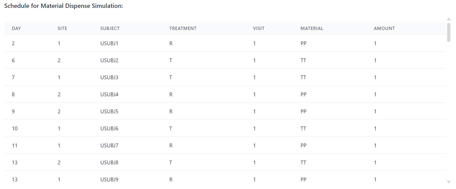
Figure 4. Monte Carlo Simulation Step A
-
Create a group of centers, add the initial supply according to the supply strategy;
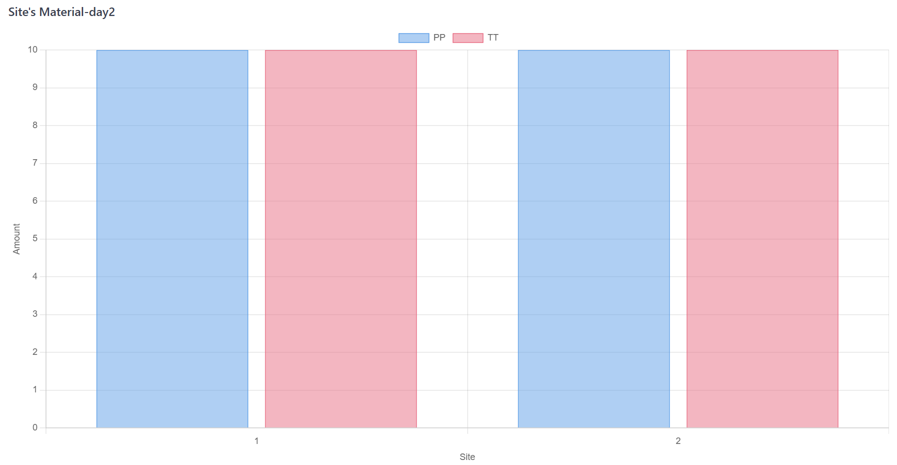
Figure 5. Monte Carlo Simulation Step B
-
Advance trial day by day, dispense the materials according to the schedule of visit;
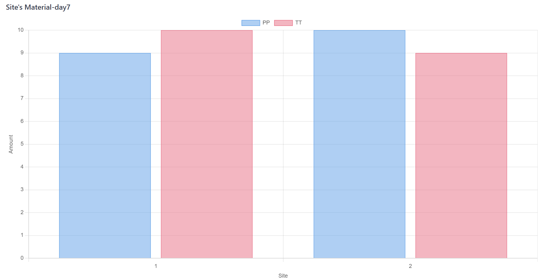
Figure 6. Monte Carlo Simulation Step C
-
Check the stock after every material dispensing. If the stock under pre-specified threshold, re-supply is triggered. The materials will be restock after shipment period;
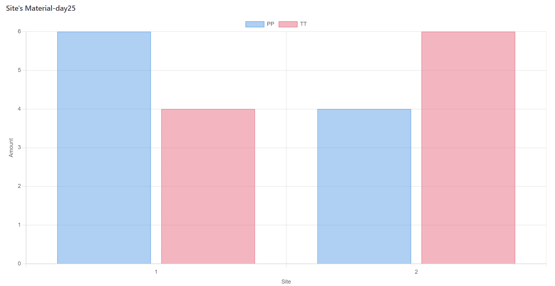
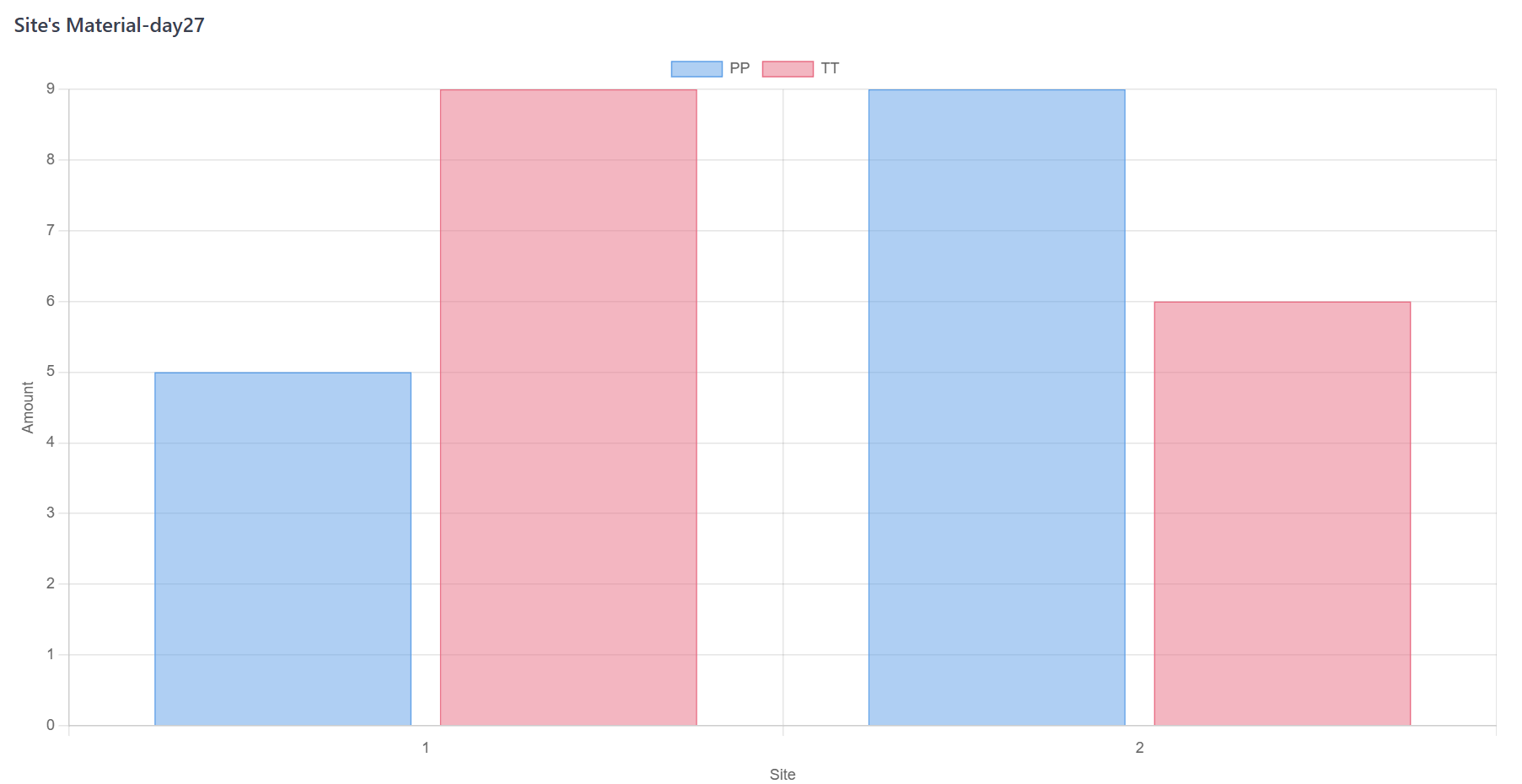
Figure 7. Monte Carlo Simulation Step D
- Run trial till the end. Anytime any center fails to dispense materials, the simulation will be recorded as failure. Otherwise, the number of supply (initial supply and re-supply) will be collected;
- Repeat A to E certain times to stablize the simulation outcomes.
3. Parameters Specification
Figure 8 presents the input panel for Simulator.
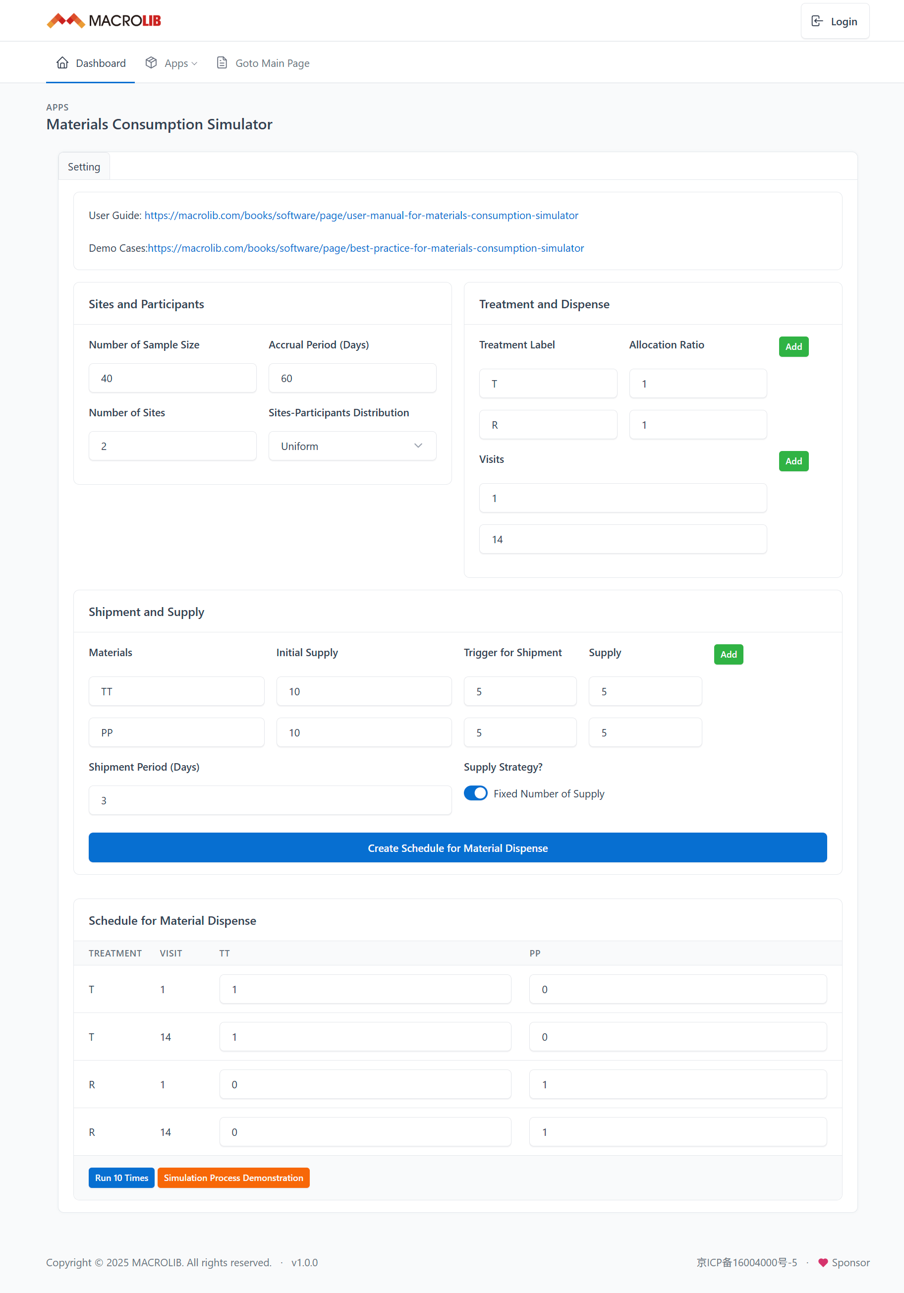
Figure 8. Input Panel
3.1. Trial Design
The trial protocol provides crucial information that forms the foundation for your simulation. From the protocol, the following key parameters are extracted:
Sample Size refers to the total number of patients to be enrolled in the clinical trial. It is essential for determining the overall scale of the trial and helps estimate material supply.
- The protocol typically defines the number of treatment arms and the allocation ratio for each arm. This allocation ratio is critical for simulating how resources and materials will be dispensed across different treatment groups. This ratio must be incorporated into the simulation to accurately predict material needs and resource distribution.
Table 2. Example of Treatment Label and Allocation Ratio
| Trial Protocol | Input Panel | ||
|---|---|---|---|
| Treatment Arm | Allocation Ratio | Treatment Label | Allocation Ratio |
| Example 1: Placebo Controlled | |||
| Test | 2 | T | 2 |
| Placebo | 1 | P | 1 |
| Example 2: Dose Ranging | |||
| Placebo | 1 | P | 1 |
| Low Dose | 1 | L | 1 |
| Mid Dose | 1 | M | 1 |
| High Dose | 1 | H | 1 |
The schedule of visits is another essential parameter. It outlines when patients are expected to visit the clinical centers throughout the trial. However, in many cases, not all visits require material dispensing. To streamline the simulation, you can simplify the schedule by focusing only on visits where material dispensing occurs. For instance: If patients are required to visit the center once a week for monitoring, but materials are only dispensed once a month, the visit schedule in the simulation can be adjusted to reflect only the monthly dispensing visits, rather than weekly visits. This simplification helps reduce unnecessary complexity in the simulation while ensuring that material dispensing events are accurately captured.
3.2. Logistic
Logistical factors, although rarely presented directly from the trial protocol, have a significant impact on the outcomes of the simulation. These factors play a crucial role in determining how materials are handled and distributed throughout the trial.
-
Materials Packaging is a critical, yet frequently under-discussed, component of trial logistics.
The mode in which materials are packaged and distributed can create entirely different scenarios in terms of material supply. For example, variations in packaging sizes can significantly affect how supplies are managed and dispensed at the centers. These variations can, in turn, impact the availability of materials, potentially influencing the study quality.
Additionally, the number of centers and the accrual period (the duration over which patients are enrolled) are key logistic factors that directly influence the patient enrollment rate and, consequently, the material dispensing process. The number of centers determines how widely the trial is distributed geographically and can affect how quickly patients are enrolled. Similarly, the accrual period dictates how long participants will be recruited, which in turn impacts when materials need to be distributed and replenished.
By taking into account these logistical components, MACROLIB ensures that the simulation reflects more realistic, real-world scenarios. This allows for a more accurate estimation of material requirements and helps in the planning of resources and timelines for trial execution.
3.3. Supply Strategy
The Supply Strategy refers to the procedures used to manage the flow of materials throughout the clinical trial. It ensures that the right quantity of materials is available at the right time and place, optimizing resource usage and reducing the risk of shortages or overstocking. This strategy is broken down into three main components: Initial Supply, Trigger for Re-supply, and Re-Supply.
3.3.1. Initial Supply
The Initial Supply refers to the amount of material that needs to be available at the start of the clinical trial to ensure that patient enrollment and treatment begin smoothly.
3.3.2. Trigger for Re-supply
The Trigger for Re-supply defines the point at which additional materials need to be shipped to the clinical trial sites. When the stock at a clinical site reaches a pre-defined minimum level, a shipment is triggered to restock the site. Shipments can take time, ensuring that materials are sent ahead of time before the stock runs low.
3.3.3. Re-Supply
Re-Supply refers to the process of restocking materials at clinical trial sites during the conduct, ensuring continuous availability of the required items. There are two major modalities:
-
Fixed Re-Supply
Users can define a fixed number of re-supply in the system. This approach can be useful when there are predictable supply needs or when the logistics team wants to maintain a consistent shipping schedule.
-
Adaptive Re-Supply
Alternatively, most of material supply system (IRT) can automatically calculate how much material needs to be restocked, based on current inventory levels and future usage projections. This approach dynamically adjusts the re-supply quantities.
Adaptive re-supply helps ensure that clinical sites are replenished with the correct amount of materials at the right time, preventing both shortages and overstocking.
3.4. Number of Simulation
To ensure the reliability and stability of the simulation outcomes, MACROLIB recommends conducting at least 100 iterations for each simulation. This helps stabilize the results and reduces the potential variability caused by random fluctuations in the data. While 100 iterations is the minimum recommended for general accuracy, the more iterations you run, the higher the reliability of the outcomes.
However, due to current resource limitations, MACROLIB only provides the option for a simulation of 10 iterations by default. This limited number is suitable for basic exploratory analysis but may not provide the full level of accuracy required for more complex simulations.
For users needing more intensive simulations or higher iteration counts, we encourage you to contact the Help Desk. Our team can assist in providing a customized solution that fits your specific simulation needs and resource requirements.
4. Intepretation
Figure 9 presents the output panel for Simulator.
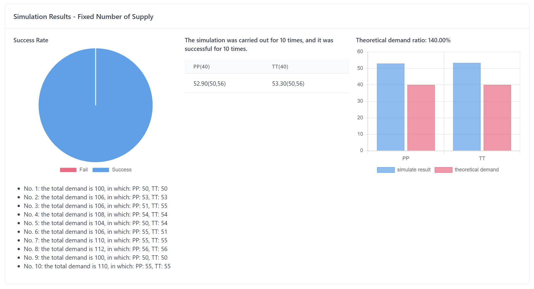
Figure 8. Input Panel
The simulation provides valuable insights to help you assess and refine your material supply strategy. ByFigure running9 multiple iterations,presents the simulationoutput deliverspanel keyfor outputsSimulator.
Figure to8. answerOutput criticalPanel
Let’s take a closer look at the two main pieces of information the simulation provides:
-
OneProbability ofthe most critical questions in trial logistics is whether your supply strategy will be able to maintain sufficient stock at each clinical site throughout the trial. The simulation helps answer this question by providing a probability of success that indicates the likelihood that your supply strategy will keep each site adequately stocked.OutstockTheThisprobability of success is calculated by running multiple simulations with different random outcomes (e.g., varying patient enrollment rates, treatment allocations, and supply chain conditions). The resultendpoint reflects the likelihood that the supply strategy you’ve chosen will ensure enough material is available at the centers.The higher the probability of success, the better your supply strategy covers the potential risks.A higher probability means that the strategy is more likely to prevent stockouts, minimize delays, and maintain compliance with the trialprotocol. Essentially, a high probability means your material distribution plan is more robust and reliable,protocol, while a low probability suggests that the strategy may need adjustments to avoid stock shortages.In short, this output provides you with a clear picture of whether your supply strategy will be able to meet the demand at clinical sites, given the expected variability in patient enrollment, shipment delays, and other logistical factors.
Utility Rate
Another critical output from the simulation is the utility rate of consumption, which compares the actual material consumption (i.e., the amount of product shipped to clinical sites) with the theoretical consumption (i.e., the amount of product actually used by patients in the trial).
Theoretical Consumption is the estimated amount of material needed based on trial parameters, such as the number of patients, treatment allocation, and visit schedule.
Actual Consumption refers to the quantity of material shipped to the clinical centers, which includes both what is used by the patients and any additional materials sent to account for uncertainties (e.g., extra stock for re-dispenses, anticipated losses, etc.).
Theoretical Consumption is the estimated amount of material needed based on trial parameters, such as the number of patients, treatment allocation, and visit schedule. Theoretical consumption assumes that there are no discrepancies in patient behavior, no delays, and no unexpected issues with supply.The ratio of actual consumption to theoretical consumption is a key metric that reflects the efficiency of your supply strategy. The utility rate is calculated conditioned on the coverage of your supply strategy. If the supply strategy has a high coverage (i.e., a high probability of success), the utility rate will give you a better idea of how much excess
or shortageof materials there might be, helping you fine-tune your shipping strategy for greater efficiency.The